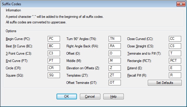
PConnect provides an easy to use and superior point-connection tool designed to combine the best features of attributed point coding with an easily controlled, yet powerful, 2D and 3D line control language. PConnect's enhanced suffix codes give the operator increased flexibility and the ability to produce automated linework and layering. PConnect can use your company's specific description keys, combined with its suffix codes, to create robust geometry from surveyed data collected in the field. The linework is drawn on specified layers as defined by a description key style file.

Two pieces of data are used to achieve the desired line work: Coordinate-data and the description key file. The field-data coordinate consists of a point number, northing, easting, elevation, and description. The description key file specifies a user-defined description to process features (lines and arcs) onto a user-specified layer name. PConnect can read coordinate data from an ASCII file (formatted as PNEZD), and Civil 3D point data.

PConnect has Three Linework Output Options:

• 2D polylines drawn at elevation 0 for planimetrics;


• 3D polylines (breaklines) drawn at the collected elevation; and


• Civil 3D survey figures drawn at the collected elevations from point data in the Survey database.

The 3D polylines and/or Civil 3D survey figures can be used to create surfaces. Essentially, PConnect creates line work by connecting points with the same code.

Examples

Click on the    icons below to view video demonstrations of these PConnect Examples
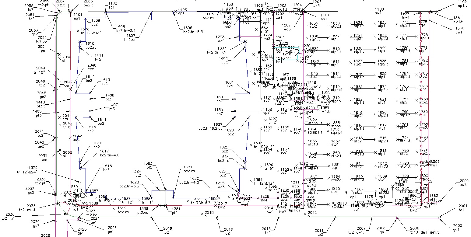
A site plan example (click on image for full size view):
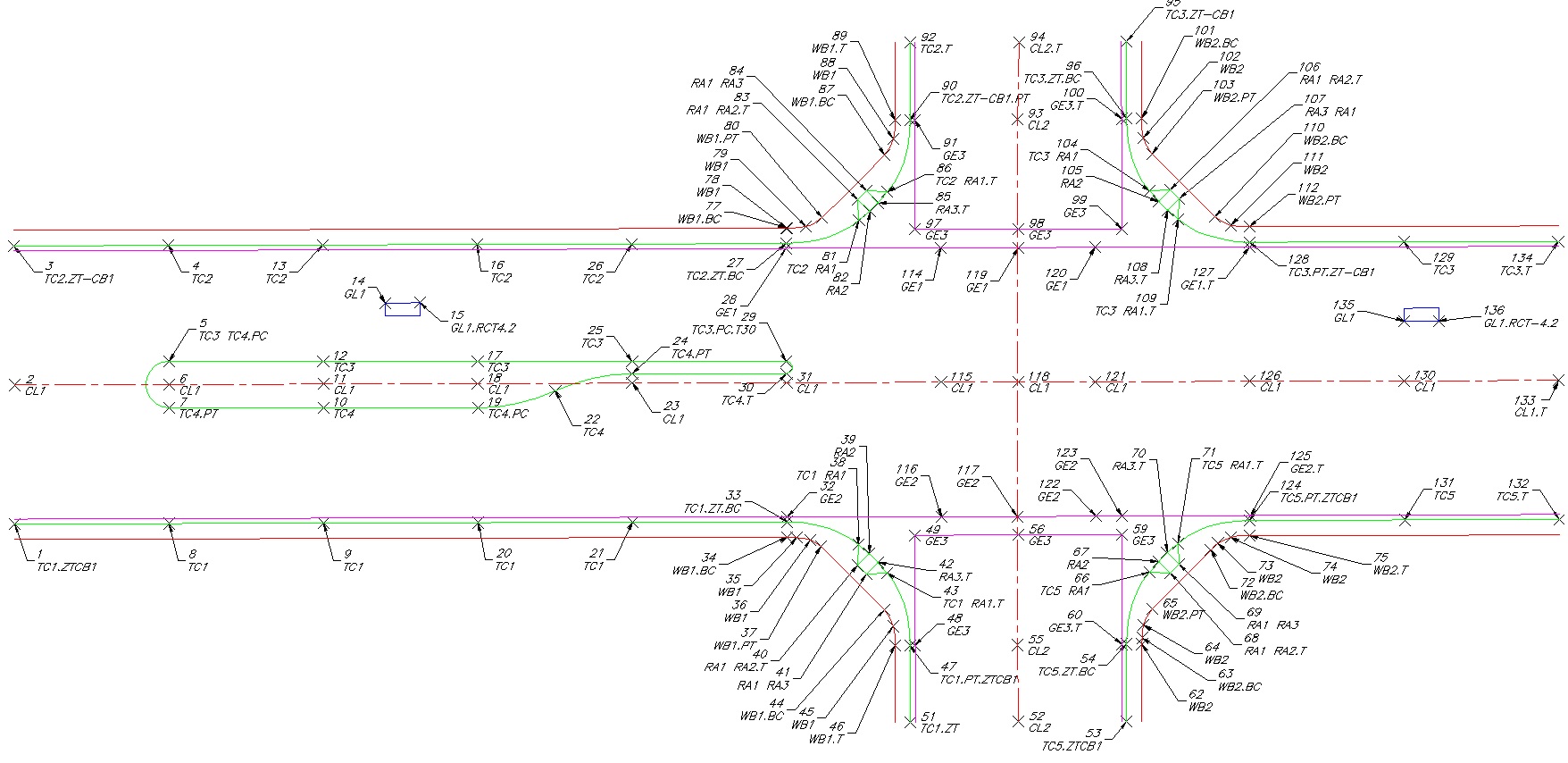
An intersection example created by PConnect using the New template suffix code (click on image for full size view):
User-defined description keys are used to separate features and line work. For example, the code, EP, could indicate edge of pavement. If there are two separate edges of pavement being collected in a cross-section method, the field personnel can indicate the right edge of pavement as "EP1" and the left edge of pavement as "EP2." PConnect will draw a separate polyline for each code. In addition, PConnect has suffix codes that the field personnel can add to the description key to instruct it to begin a curve, end a curve, end a polyline, recall a previous point, and close a polyline. With the combination of description keys and suffix codes, field personnel can reuse EP1 once a previous EP1 has been terminated with the correct suffix code.

Straight Segment Suffix Codes

• Straight Segments: When there is not a suffix code, straight segments are created.


• Close Straight: Closes a polyline back to the starting point using a straight segment.


• Square: Draws a square polyline (4-sided polygon).


• Turn 90° Angle: Adds straight segments turned at 90° angles from the previous segment.


• Right Angle Back: Calculates two straight segments forming a right angle.


• Rectangle: Creates a closed rectangle from two points (with an offset distance) or closes back to the starting point at a right angle when three (3) or more points are used.


• Extend: Extends or shortens a straight segment along the bearing of the point with the code and the previous point.

• Begin Curve: Creates a tangent curve from the last segment.


• 3 Point Curve: Creates a non-tangent curve using three (3) points.


• Best Fit Curve: Creates a Best Fit Curve passing through all the points with the same description.


• Close Curved: Closes the current polyline back to the starting point with a tangent curve.


• Circle: Draws a circle at the radius.


• End Curve: Stops curve calculation and begins straight segments.

Offset Suffix Codes:

• Offset: Offset polylines to either the right, with a positive distance, or to the left, with a negative distance.


• Middle: Offset polylines on both the right and left sides of the collected points at half (1/2) the specified distance.


• Template: Offset multiple polyline based on a user-defined template.

Examples:

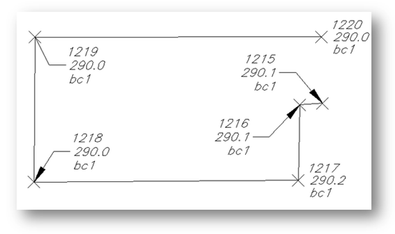
Straight Segments

• The default connection between points, without any specific suffix code, is a straight segment. 
• The polyline, BC1, is drawn starting at point 1215, continuing through points 1216, 1217, 1218, 1219, and ending at point 1220.

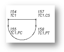
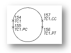
Close Polyline with Straight Segment (.CS)

• To close geometry back to the starting point with a straight segment, add the description suffix Close Straight (.CS).
• The polyline, TC1, is drawn starting at point 154, continuing through points 155, 156, and 157 where it encounters the Close Straight (.CS) code, and a final segment is drawn back to the starting point 154.

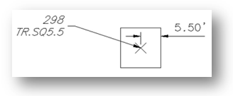
Square Example

• To draw a square at a point, use the square suffix code and an offset distance value.
• The distance (#) must be entered after the square code (.SQ#).
• The square code can be added to a single description (TR.SQ5.5), and a square polyline (polygon with 4 sides) will be drawn, or it can be one of the multiple descriptions added to a point (EG1 HM.CR5.5).

Turn 90° Angles Example

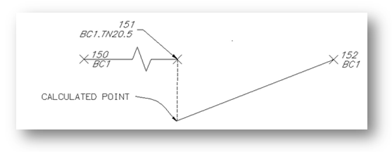
A single distance following the code:

• The polyline, BC1, is drawn starting at point 150, continuing to point 151, and encounters the Turn 90° Angles (.TN) code.  
• The code is followed by one distance (20.5); one segment will be added between point 151 and point 152.  
• Since the distance is a positive number, the segment will be at a right angle to the previous segment and turning to the right (CW) 20.5 units. From this new point, a segment is drawn continuing to point 152.

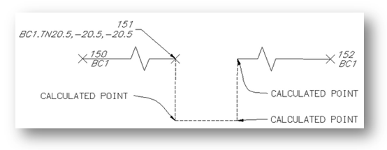
Multiple distances following the code:

• The polyline, BC1, is drawn starting at point 150, continuing to point 151, and encounters the Turn 90° Angles (.TN) code.
• Since the code is followed by three distances (20.5,-20.5,-20.5) separated by commas, three additional straight segments will be added between points 151 and 152.
• The first segment is drawn at a right angle from the previous segment to the right (CW) at 20.5 units since the distance (#) is a positive value.
• The second segment is drawn at a right angle from the first segment to the left (CCW) at 20.2 units since the distance (#) is a negative value.
• The third segment is drawn to the left from the previous segment at 20.5 units again.
• From this last calculated point, point connection continues sequentially to point 152.

Note:    The code assumes the previous segment was a straight segment, and this suffix code is ignored if in the middle of any of the curve suffix codes.  This code can be combined with a termination code (.T, .CS, or .CC).

Right Angle Back Example

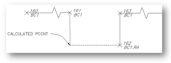
• To calculate a hidden point, which is at right angles to two known points, use the Right Angle Back suffix code.
• The polyline, BC1, is drawn starting at point 160, continuing to point 162, where it encounters the Right Angle Back code.
• The code instructs PConnect to calculate a right angle back from the previous two points of 160 and 161, the current point 162, and the following point 163 as the straight segments to calculate the starting bearings for the right angle point.
• The right angle point is placed between point 162 (point with the code) and the previous point 161.

Note:    This suffix code requires at least two prior points to calculate the starting angle and at least one point to calculate the ending angle.  If there is no solution, parallel lines, or the calculated point is too far away, a straight line is drawn between the two points and a warning message is displayed at the end.

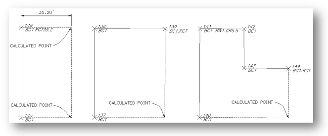
Rectangle Examples

• To draw a rectangle or a closed polyline with a right angle calculation point, use the rectangle suffix code.
• To calculate a rectangle using only two points, an offset distance (#) must be entered after the rectangle code (.TN#).
• If there are three or more points, any offset distance value will be ignored, and the command will attempt to calculate a right angle point from the end and starting points of the polyline.
• The command will assume the first segment was a straight segment and the last segment was a straight segment.

Extend Examples

• To extend a point a given distance (e.g., something is obscuring an object’s corner), use the Extend (.E#) code.
• If the given distance (#) is positive, the point will move the given distance along the angle (bearing) created from the previous point.
• If the given distance (#) is negative, the point will be moved back (straight segment shorten) along the angle (bearing) created from the previous point.

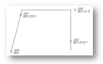
Example of Extend with Both Positive and Negative Distances

• A polyline, BO1, is drawn starting at point 200, continuing to point 201, where it encounters the Extend (.E) code.
• Since the code is followed by a positive distance (5.5), the straight segment between point 200 and point 201 is extended 5.5 units.
• The polyline continues from this calculated point to the next point 202, where it encounters an Extend (.E) code with a negative number.
• A straight segment is now drawn from the previously calculated point (not from the coordinates of point 201) to a location 5.0 units short of point 202.
• The polyline continues from this point towards the next point 203, where it encounters a point with two codes, Extend (.E) and Terminate (.T).
• A straight segment is drawn from the previously calculated point toward 203, extends past it 10.0 units, and because of the Terminate (.T) code, B01 ends at this location.

Example of Extend Using a Negative Distance

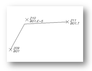
• A polyline, BO1, is drawn starting at point 209, continuing to point 210, where it encounters the Extend (.E) code.
• Since the code is followed by a negative distance (-5), the straight segment between point 209 and point 210 is shortened 5.0 units.
• The polyline continues from this calculated point and ends at point 211, where it encounters a Terminate (.T).

Curve Example Using .PC (2 Point Tangent Curve)

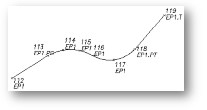
• The polyline, EP1, is drawn starting at point 112 and continues to point 113 with the Begin Curve (.PC).
• A tangent curve is calculated from point 113 to point 114 from the bearing along the point 112 to point 113.
• Curve segments are created between points 114 and 115, 115 and 116, 116 and 117, 117 and 118 and are all tangent to the proceeding curve segment.
• The End Curve (.PT) code is encountered at point 118, and a straight segment is drawn between points 118 and 119.
• The polyline ends at point 119.

Note:    Field crews do not have to add a description suffix at a point of reverse or compound curve.  As long as there is not a straight segment, do not add the End Curve (.PT) code, and the command will draw the reverse or compound curve segments.  PConnect checks for direction changes between segments and automatically determines the presence of a PRC or PCC, therefore, there is no need to identify the PRC or PCC with a PT/PC.

Curve Example Using .C3 (3 Point Non-Tangent Curve)

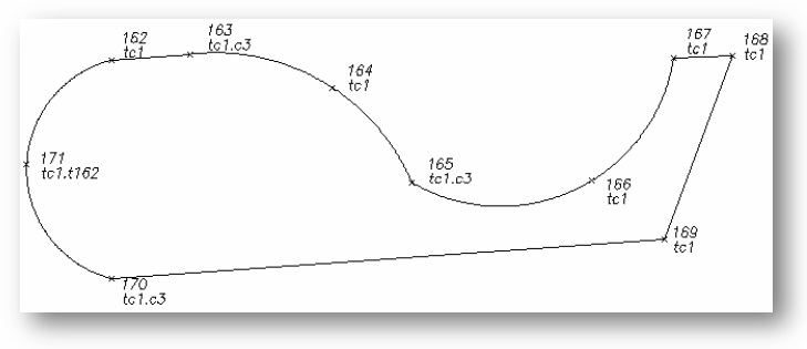
• The polyline, TC1, is drawn starting at point 162 and continues to point 163 with the 3 Point Curve (.C3).
• A non-tangent 3 Point Curve is drawn starting at point 163, through points 164 and 165.
• A 3 Point Curve (.C3) code is encountered at point 165.
• Another non-tangent 3 Point Curve is drawn starting at point 165, through points 166 and 167.
• An End Curve (.PT) was not needed at point 165 or point 167 to end the 3 Point Curve.
• At point 167, straight segments begin continuing through points 168, 169, and 170.
• At 170, the last 3 Point Curve (.C3) code is encountered, and the next two points are used.
• In this case, the second point 162 has the Terminate to # (.T162), so the points 171 and 162 are used to calculate the 3 Point Curve.
• The polyline ends at point 162.

Note:    Field crews do not have to add a description suffix at a point of reverse or compound curve, since the .C3 suffix code only reads 3 consecutive points.  Field personnel can add a new C3 to start a new 3 Point Curve.  PConnect checks for direction changes between segments and automatically determines the presence of a PRC or PCC, so there is no need to identify the PRC or PCC when using the C3 suffix code.  See point numbers 162 - 171 above.

Curve Example Using Best Fit Curve (.BC) (Best Fit Non-Tangent Curve)

• The polyline, TC1, is drawn starting at point 173, and continues to point 174 where the Best Fit Curve (.BC) code is encountered.
• Starting at point 174, TC1 continues through points 175, 176, 177, 178, 179, 180, and ends at point 181.  
• A Best Fit Curve is calculated passing through each of the points.
• At point 181, straight segments begin continuing through points 182, 183, 184, and 185.
• At 185, a Best Fit Curve (.BC) code is encountered; at point 186, a Terminate code is encountered.
• Because this leaves only two points to calculate a curve, and the best-fit method requires at least three (3) points, PConnect tries to use the (.PC) tangent curve method.
• Since there is a segment before point 185, PConnect calculates the curve between points 185 and 186 using the tangent curve (.PC) method.
• The polyline then ends at point 186.

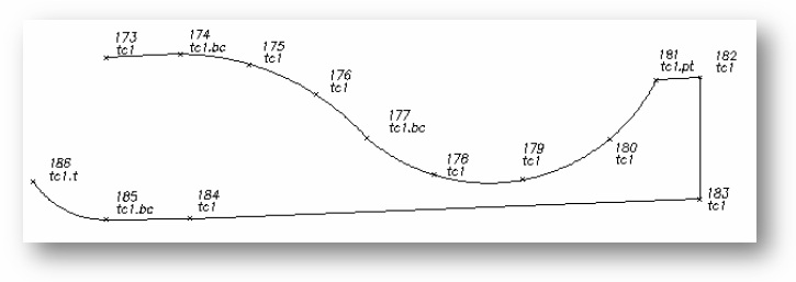
Note:    If only two points are encountered after the Best Fit Curve (.BC) code and the bearings created between the first two points and the second two points differ by less than five (5) degrees, the Begin Curve (.PC) calculation method is used to create a reverse curve.  If the Best Fit Curve method was used, the curved segments would appear almost like two straight segments.

 Close Polyline with Curve (.CC)

• To close geometry back to the starting point with a curve segment, add the description suffix Close Curved (.CC).
• The polyline, TC1, is drawn starting at point 154, continues through points 155, 156, and 157 where it encounters the Close Curved (.CC) code, and a final segment is drawn back to the starting point 154 as a tangent curve using the last segment 156 and 157 to calculate the curve.

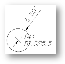
Circle Example

• To draw a circle at a point, use the Circle suffix code and a radius value.  The radius (#) must be entered after the Circle code (.CR#).
• The Circle code can be added to a single description (TR.CR5.5), and a circular polyline (polygon with multiple sides) will be drawn, or it can be one of the multiple descriptions added to a point (EG1 HM.CR5.5).

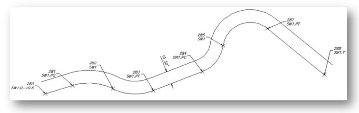
Example of Offset along a Path

• A polyline, SW1, is drawn starting at point 280 and ending at point 288, creating curves and lines per the encountered suffix codes.
• The offset polyline, SW1, is drawn at 10.5 units to the right side of the original path of the collected point starting at point 280 and ending at point 288, creating curves and lines per the encountered suffix codes.

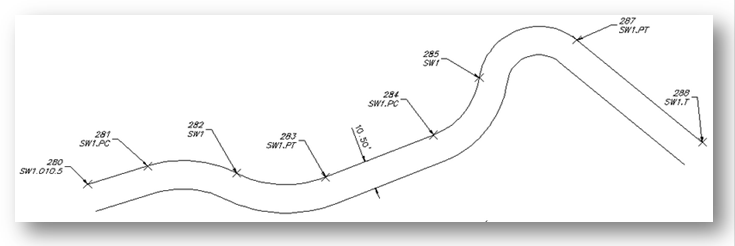
Note:  The offset polylines will create a fillet with a zero (0) distance if the offset is larger than a calculated curve radius.

• A polyline, SW1, is drawn starting at point 280 and ending at point 288, creating curves and lines per the encountered suffix codes.
• The offset polyline, SW1, is drawn at 10.5 units to the left side of the original path of the collected point, starting at point 280 and ending at point 288, creating curves and lines per the encountered suffix codes.

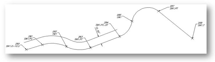
Example of Offset Stopping before the End of the Original Path

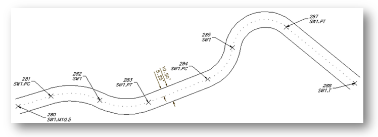
• A polyline, SW1, is drawn starting at point 280 and ending at point 288, creating curves and lines per the encountered suffix codes.
• The offset polyline, SW1, is drawn at 10.5 units to the left side of the original path of the collected point, starting at point 280 and ending at point 284, where it encounters the Offset Terminate (.OT) code.

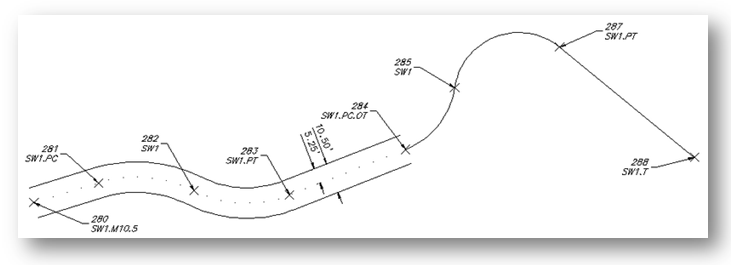
Example of Offset Where the Offset Distance Changes

• A polyline, SW1, is drawn starting at point 280 and ending at point 288, creating curves and lines per the encountered suffix codes.
• The first offset polyline, SW1, is drawn at 10.5 units to the left of the original path of the collected point starting at point 280 and ending at point 284 when it encounters the second Offset (.O5.25) code.
• The second offset polyline, SW1, is drawn at 5.25 units to the right of the original path of the collected point starting at point 284 and ending at point 288 when it encounters the Terminate (.T) code.

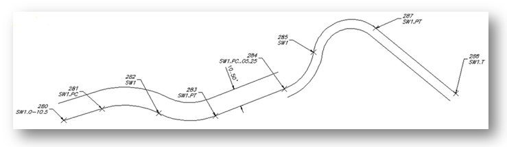
Note:    There is not a transition from the first Offset code offset distance (-10.5) to the second Offset code offset distance (5.25); the first one stops, and the second one begins.

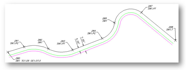
Example of Multiple Offsets to Different Layers

• The first point along the SW1 path has three description keys.
• The second and third description keys have the Offset (#) code.
• A polyline, SW1, is drawn starting at point 280 and ending at point 288, creating curves and lines per the encountered suffix codes.
• The first offset polyline, TC1, is drawn at 5 units to the right side of the original path on the layer specified by the TC# description key in the Description Key Style file.
• The second offset polyline, GE1, is drawn at 7.5 units to the right side of the original path on the layer specified by the GE# description key in the description key style file.

Example of Middle along a Path

• The offset polylines, SW1, are drawn at 5.25 units each side of the original path of the collected point starting at point 280 and ending at point 288, creating curves and lines per the encountered suffix codes.

Note:    The offset polylines will create a fillet with a zero (0) distance if the offset is larger than a calculated curve radius.

Example of Middle Stopping before the End of the Original Path

• The offset polylines, SW1, are drawn at 5.25 units each side of the original path of the collected point starting at point 280 and ending at point 284, creating curves and lines per the encountered suffix codes.
• It encounters an Offset Terminate (.OT) code at point 284.
• The offsets end and a single polyline is drawn starting at point 284, continuing through points 285, 287, and ending at point 288.

Example of Middle Change Offset Distance before the End of the Original Path

• The offset polylines, SW1, are drawn at 5.25 units each side of the original path of the collected point starting at point 280 and ending at point 284, creating curves and lines per the encountered suffix codes.
• It encounters another Middle (.M18.5) code at point 284.
• The second set of offset polylines, SW1, are drawn at 9.25 units each side of the original path of the collected point starting at point 284 and ending at point 288, creating curves and lines per the encountered suffix codes.

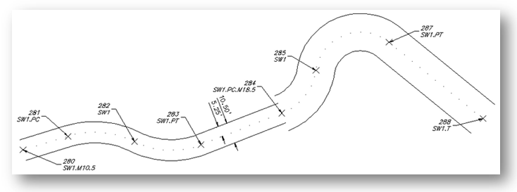
Note:    There is not a transition from the first Middle code offset distance (10.5) to the second Middle code offset distance (18.5); the first one stops, and the second one begins.

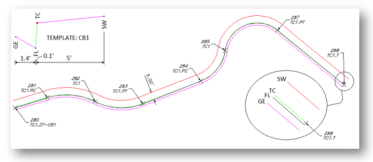
Example of a Template along a Path

• The template CB1 has three offsets.  The first offset, SW, is 5.0 units to the right of the field shot point (red dot, TC).  The second offset, FL, is 0.1 units to the left of the field shot point.  The third offset, GE, is 1.4 units left of the second offset.
• The polyline, TC1 (green line), is drawn starting at point 280 and ending at point 288, creating curves and lines per the encountered suffix codes.
• A first offset polyline, SW1 (red line), is drawn at 5.0 units to the right of the original path of the collected point, starting at point 280 and ending at point 288, creating curves and lines per the encountered suffix codes.
• A second offset polyline, FL1 (black line), is drawn at 0.1 units to the left of the original path of the collected point, starting at point 280 and ending at point 288, creating curves and lines per the encountered suffix codes.
• A third offset polyline, GE1 (magenta line), is drawn at 1.5 (0.1 + 1.4) units to the left of the original path of the collected point, starting at point 280 and ending at point 288, creating curves and lines per the encountered suffix codes.

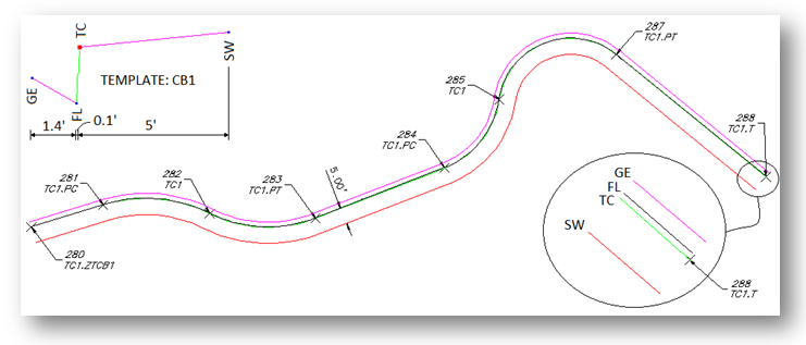
Note:     The offset polylines will create a fillet with a zero (0) distance if the offset is larger than a calculated curve radius.

Example of a Template along a Path Mirrored

• The template CB1 has three offsets.  The first offset, SW, is 5.0 units to the right of the field shot point (red dot, TC).  The second offset, FL, is 0.1 units to the left of the field shot point.  The third offset, GE, is 1.4 units left of the second offset.
• When a "-" negative character is added between the Template code (.ZT) and the template name (#), the template offset distances are mirrored (reversed) about the field shot point (red dot) in the template.
• The polyline, TC1 (green line), is drawn starting at point 280 and ending at point 288, creating curves and lines per the encountered suffix codes.
• A first offset polyline, SW1 (red line), is drawn at 5.0 units to the left of the original path of the collected point starting at point 280 and ending at point 288, creating curves and lines per the encountered suffix codes.
• A second offset polyline, FL1 (black line), is drawn at 0.1 units to the right of the original path of the collected point starting at point 280 and ending at point 288, creating curves and lines per the encountered suffix codes.
• A third offset polyline, GE1 (magenta line), is drawn at 1.5 (0.1 + 1.4) units to the right of the original path of the collected point starting at point 280 and ending at point 288, creating curves and lines per the encountered suffix codes.

Example of a Template Change along a Path:

• The template, CB1, has three offsets.  The first offset, SW, is 5.0 units to the right of the field shot point (red dot, TC).  The second offset, FL, is 0.1 units to the left of the field shot point.  The third offset, GE, is 1.4 units left of the second offset.
• The template, CB3, has three offsets.  The first offset, SW, is 5.0 units to the right of the field shot point (red dot, TC).  The second offset, FL, is 0.1 units to the left of the field shot point.  The third offset, GE, is 1.4 units to the left of the second offset.
• The polyline, SW1, is drawn starting at point 280 and ending at point 288, creating curves and lines per the encountered suffix codes.
• A first offset polyline, SW1, is drawn at 10.5 units to the left of the original path of the collected point starting at point 280 and ending at point 284 when it encounters the second Offset (.O5.25) code.
• A second offset polyline, SW1, is drawn at 5.25 units to the right of the original path of the collected point starting at point 284 and ending at point 288 when it encounters the Terminate (.T) code.

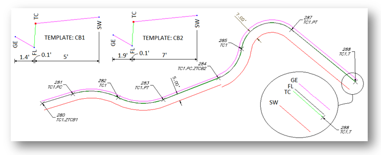
Note:     There is not a transition from the first Template to the second Template; the first one stops, and the second one begins.

Example of Elevation Change on Offset Using the 3D Polylines Draw Option:

• The Elevation on Offset (.Z#) code adjusts the collected elevation of a point by the height (#) value.
• A 3D polyline, SW1, is drawn starting at point 280 and ends at point 288, creating curves and lines per the encountered suffix codes and at the elevations associated to the points.
• The offset 3D polyline, SW1, is drawn at 5.5 units to the left of the original path of the collected points, starting at point 280 and ending at point 288, creating curves and lines per the encountered suffix codes and at the adjusted elevations of 0.3.
• Note the elevations at points 280, 283, 285, and 288.
• The elevations along the original path are the same as the elevation of the associated point, but the elevations along the offset 3D polyline are 0.3 higher than the elevation associated to the original point.

Example of Elevation Change on Offset Using the 3D Polylines Draw Option:

• Using the same points from above, but with one modification to the description of point 284, the elevation on Offset (.Z) suffix code is added without an adjustment value.
• A 3D polyline, SW1, is drawn starting at point 280 and ending at point 288, creating curves and lines per the encountered suffix codes and at the elevations associated to the points.
• The offset 3D polyline, SW1, is drawn at 5.5 units to the left of the original path of the collected points.
• Starting at point 280 through point 283, the elevations on the offset 3D polyline have been adjusted higher by 0.3 units. 
• Starting at point 284 through point 288, the elevations on the offset 3D polyline are the same as the associated point.

Note:    Like all elevations between points on a 3D polyline, there is a linear interpolate of the elevations on the offset 3D             polyline between points 283 and 284.

Example of Elevation Change on Offset Using the 3D Polylines Draw Option:

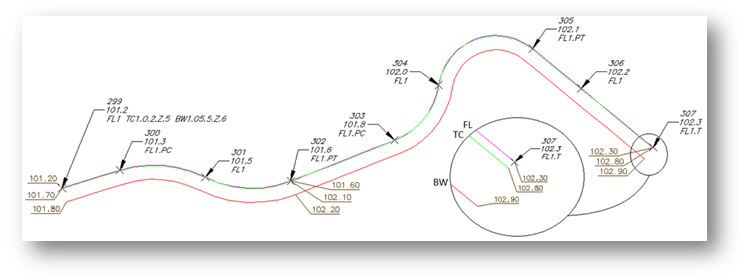
• A third example uses three (3) description keys, with the second and third description keys having both an offset (.O#) and an Elevation on Offset (.Z#) suffix code.
• A 3D polyline, FL1, is drawn starting at point 299 and ending at point 307, creating curves and lines per the encountered suffix codes and at the elevations associated to the points.
• The first offset 3D polyline, TC1, is drawn at 0.2 units to the right of the original path of the collected points with elevations 0.5 units higher than the elevations of the associated points.
• The second offset 3D polyline, BW1, is drawn at 5.5 units to the right of the original path of the collected points with elevations 0.6 units higher than the elevations of the associated points.

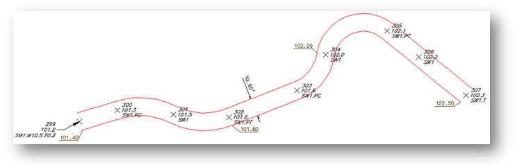
Example of Elevation Change on Middle Using the 3D Polylines Draw Option:

• The Elevation on Offset (.Z#) code adjusts the collected elevation of a point by the height (#) value.
• No 3D polyline is drawn along the original path when using the Middle suffix code.
• Two offset 3D polylines, SW1, are drawn at 5.25 units each side of the original path of the collected points starting at point 299 and ending at point 307, creating curves and lines per the encountered suffix codes.
• The elevations on the offset 3D polylines are 0.2 units higher than the elevations associated to the original points.

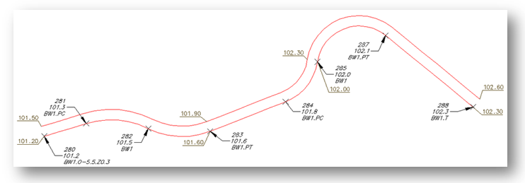
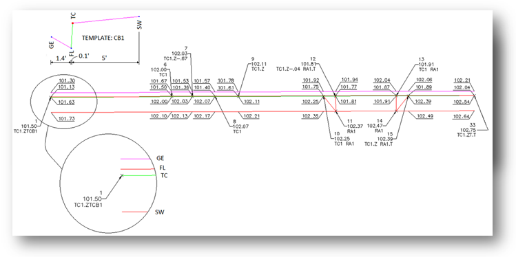
Example of Elevation Change on Template:

• The Elevation on Offset (.Z#) code replaces the green segment's height (as displayed in the PConnect Template Manager) with the height (#) on the code.
• A 3D polyline, TC1, is drawn starting at point 1, through points 6, 7, 8, 9, 10, 12, 13, and ends at point 33 at the elevations associated to the points.
• From the template, three additional offsets are specified, GE, FL, and SW.
• SW is 5.0 units to the right and 0.1 units higher than TC1.
• FL is 0.1 units to the left and 0.5 units lower than TC1.
• GE is 1.4 units to the left and 0.17 units higher than FL.
• At point 7, notice the Elevation on Offset (.Z-.67).  The -0.5 height defined in the template (green segment) will be replaced with -0.67, due to a curb inlet, and will continue through point 8.
• At point 9, notice the Elevation on Offset (.Z) without a value.  The temporary height of -0.67 for the green segment returns to the defined height of -0.5.
• Compared to the associated elevations of TC1, the 3D polylines drawn along the FL between points 6 and 7 transition from -0.5 at point 6 to -0.67 at point 7 and transition between points 8 and 9 from -0.67 to -0.05.
• At point 10, notice the two description keys, TC1 and RA1.  A 3D polyline drawn along RA starts at point 10, continues through point 11, and ends at point 12, which also has two description keys, TC1 and RA1.T.
• At point 12, notice the Elevation on Offset (.Z-.04).  The -0.5 height defined in the template (green segment) will be replaced with -0.04, due to a driveway, and will continue through point 14.
• At point 15, notice the Elevation on Offset (.Z) without a value.  The temporary height of -0.04 for the green segment returns to the defined height of -0.5.
• The 3D polylines drawn along the FL between points 10 and 12 transition from -0.5 at point 10 to -0.04 at point 12, compared to the associated elevations, and transition between points 13 and 14 from -0.04 to -0.05.
• The elevations on the offset 3D polylines, SW, are 0.1 higher than the elevations associated to the original points.  

Terminate and Description Keys:

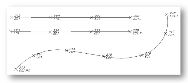
• PConnect creates a polyline along points with a common description.
• Once the Terminate code has been added to a description (e.g., EC1.T), the next time EC1 is used, a new polyline is started.  In the examples below, three separate polylines are drawn using the same description key of EC1, and they are terminated at points 218, 222, and 226 because of the added Terminate code (.T).

Terminate to Point Number Examples:
The Terminate suffix code can be followed by a point number.  When the Terminate suffix code is followed by a point number (#), it terminates at the specified point.  This allows a non-sequential or previous point to be added to the end of a polyline.  The description of the specified point is ignored.

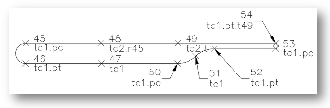
• In the example below, the point number 54 has two suffix codes, the End Curve (.PT) and the Terminate to # (.T49).
• The curve started at point number 53 and ends at point number 54; and the polyline started at point number 45 and ends at point number 49.
• Also, note the recall to point number (.R45) at point 48.
• A second polyline is drawn starting at point 45, continues through point 48, and ends at point 49.

Note:      To use these options, the field crew will have to note the point numbers used with the Terminate and Recall suffixes.

Example using Cross Section Method of Collecting Points:

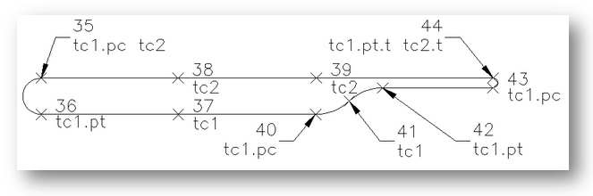
• The first polyline, TC1, is drawn starting at point 35, continuing through points 36, 37, 40, 41, 42, 43, and ending at point 44 (TC1.PT.T).
• The second polyline, TC2, is drawn starting at point 35 (second description key at point 35), continuing through points 38, 39, and ending at point 44 (TC2.T).

Terminating Linework and Recalling a Point Example
Examples of drawing a trash enclosure using three different methods are provided below.

Example of Using Two Points Collected at the Same Location:

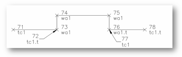
• The first polyline, TC1, is drawn starting at point 71 and ends at point 72.
• The second polyline, WA1, is drawn starting at point 73 (a second point collected at the same location as point 72), continues through points 74, 75, and ends at point 76.
• The third polyline, TC1, is drawn starting at 77 and ends at point 78.

Example of Same Geometry Using Recall Point Number: (.R#)

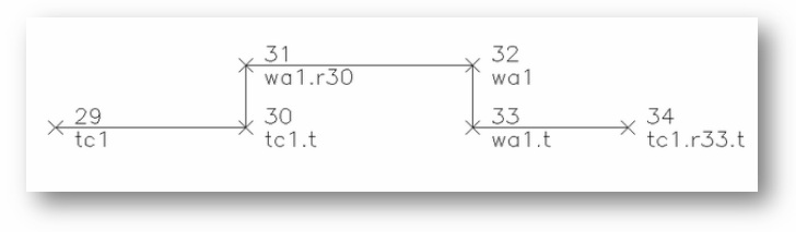
• The first polyline, TC1, is drawn starting at point 29 and ending at point 30.
• The first point number with the WA1 description key is point 31; but with the recall at # (.R30), the second polyline is drawn starting at point 30, continues through the points 31, 32, and ends at point 33.
• The third polyline, TC1, only has one point 34, but with the recall at # (.R33), a polyline will be drawn starting at point 33 and ending at point 34.

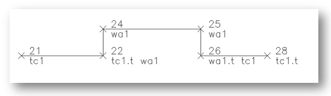
Example of Same Geometry Using Multiple Descriptions at a Single Point:

The final example uses multiple description keys at a single point.

• The first polyline, TC1, is drawn starting at point 21 and ending at point 22.
• The second polyline, WA1, is drawn starting at point 22 (due to the second description key), continues through points 24, 25, and ends at point 26.
• The third polyline, TC1, is drawn starting at point 26 and ending at point 28.

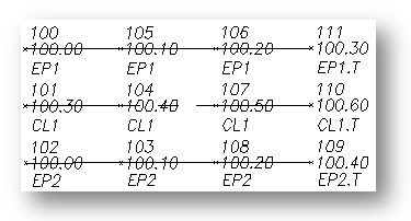
A Simple Cross-Section Example:
In this simple example, the field crew is collecting edge-of-pavement (EP#) on either side of the street.  As long as each EP has a unique number (#), PConnect processes each as a separate description key.  PConnect still processes point numbers in ascending order but makes a distinction between EP1 and EP2.

• The first polyline, EP1, is drawn starting at point 100, continues through points 105, 106, and ends at point 111 where it encounters the Terminate (.T) code.
• The second polyline, CL1, is drawn starting at point 101, continues through points 104, 107, and ends at point 101 where it encounters the Terminate (.T) code.
• The third polyline, EP2, is drawn starting at point 102, continues through points 103, 108, and ends at point 109 where it encounters the Terminate (.T) code.